Fine-Tuning | Quantize | Infer — Qwen2-VL mLLM on Custom Data for OCR: Part 3
Quantization | Inference of custom Qwen2-VL-2B mLLM
This is the 3rd Part of my three-part Qwen2-VL fine-tuning and quantization series. If you want to learn more about how to prepare a custom training dataset and fine-tune the Qwen2-VL model, go through the first 2 parts where I have explained it in depth.
Blog Series :
- Custom Dataset Preparation for multimodel LLM fine-tuning(Qwen2-VL)
- LoRA Fine-Tuning Qwen2-VL
- Quantization and Inferencing of custom Qwen2-VL-2B mLLM (GPTQ and AWQ) (This Blog)
In this blog, I will focus on the quantization of our fine-tuned Qwen2-VL model. Qwen2-VL as of now supports only two quantization methods: Activation-aware Weight Quantization (AWQ) and Generative Pre-trained Transformer Quantization (GPTQ) . I have used both methods to quantize our model and have shared my observations in this blog.
Note : Only GPTQ inference code is available now. Will up the inference code for AWQ quantization soon.

That’s nice, but why do we need to put our model on a number scale?
Let's first calculate how much GPU is ideally required to run our fine-tuned model. Here is a popular formula to calculate the GPU required to infer an LLM.

- M: GPU memory required for inference, measured in gigabytes (GB).
- P: Number of parameters in the model.
- 4B: 4 bytes (equivalent to 32 bits), representing the memory used to store each parameter.
- 32: The number of bits in 4 bytes.
- Q: The target number of bits to use per parameter for loading the model (e.g., 16 bits, 8 bits, or 4 bits).
- 1.2: Represents a 20% overhead of loading additional things like activation in GPU memory.
For the Qwen2-VL fine-tuned model (16 bits), the total GPU memory required solely for model loading is calculated as follows:
M = (2*4)(16/32) * 1.2 = 4.8 GB
Therefore, we practically require at least a 6 GB GPU to load and infer our model. While this may not seem like a significant amount, achieving a 4-bit quantized model could potentially reduce our GPU requirements. The calculation to load a 4-bit model is:
M = (2*4)(4/32) * 1.2 = 1.2 GB
This represents a theoretical reduction of approximately 75% in GPU memory requirements. In practice, we could utilize a 4 GB Nvidia GPU, which would lead to a 50% decrease in our GPU requirements.
Now that we understand the importance of quantization, let’s delve into the process of quantizing our fine-tuned Qwen2-VL model.
What is the quantization of LLM?
Quantization of large language models (LLMs) is the process of reducing the precision of the model’s weights and activations, typically from 32-bit floating-point to lower-bit representations (like 8-bit or 4-bit). This reduces the model’s memory footprint and computational requirements, allowing it to run faster and on less powerful hardware while maintaining a similar level of performance.
Activation-aware Weight Quantization (AWQ)
Traditional quantization reduces the model size by lowering the precision of weights (model parameters) from high-precision formats (e.g., 16-bit floating point) to smaller sizes (like 8-bit or 4-bit integers). While this approach saves memory, it often applies the same precision to all weights, risking accuracy loss — similar to uniformly compressing an image and losing essential details.
AWQ takes quantization a step further by recognizing that not all weights contribute equally to model accuracy. AWQ identifies and protects the most crucial weights — those linked to higher activations (output values that significantly impact predictions). During compression, these weights are retained in higher precision, while less critical weights are compressed more aggressively, preserving the model’s predictive power.
The AWQ process begins with an analysis of activation statistics, collected during a calibration phase. These statistics reveal which weights impact the model’s outputs the most. AWQ uses this insight to apply per-channel scaling, where scaling factors are determined based on activation data. This targeted approach enables efficient memory use without compromising essential performance. For example, in a model like Qwen2-VL, which processes both vision and language tasks, AWQ ensures that weights critical to both modalities are protected, maintaining performance in both areas.
AWQ works by compressing only the parts of a model that aren’t crucial for accuracy while keeping the important parts in high detail. It does this by running the model on real data during a setup phase, where it measures the outputs (called activations) of each layer. This helps pinpoint which weights (the model’s numbers) are essential for accurate results, so that only the less important weights are compressed, preserving overall performance.
How to quantize our fine-tuned Qwen2-VL model using AWQ
If you go through the official Qwen2-VL repository, they have mentioned how to use AutoAWQ for quantization. I have used the same and here is what we have to do.
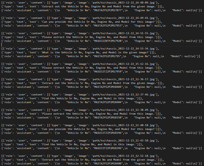
First, we need to create our calibration dataset which is just a small subset of our training dataset. The format is mentioned below.
dataset = [
    [
        {
            "role": "user",
            "content": [
                {"type": "image", "image": "file:///path/to/your/vinplate.jpg"},
                {"type": "text", "text": "Extract out the Vehicle Sr No, Engine No and Model from the given image."},
            ],
        },
        {"role": "assistant", "content": "{\n    "Vehicle Sr No": "MA1TA2YS2P2M17877",\n    "Engine No": null,\n    "Model": null\n}"},
    ],
    ...,
]
I have used around 10 images to calibrate our model for quantization. So the final combined file will be a text file with 10 samples of the same format as mentioned above. Let's name this file caliber_dataset.txt
Note: You can also create a JSON file for the same and load it accordingly.
Next, we need to set up our environment for the quantization of our model.
Clone and install the following repository from the source
git clone https://github.com/kq-chen/AutoAWQ.git
cd AutoAWQ
pip install numpy gekko pandas
pip install -e .
Note: There are additional specific requirements that need to be installed. I’ll compile a complete list, which I’ll share here once it’s ready.
Now, use the following script to load our fine-tuned Qwen2-VL model and quantize it using this caliber dataset.
from transformers import Qwen2VLProcessor
from awq.models.qwen2vl import Qwen2VLAWQForConditionalGeneration
from qwen_vl_utils import process_vision_info
import json
import ast
import torch
torch.cuda.empty_cache()
import os
os.environ['CUDA_VISIBLE_DEVICES'] = '0'

# Specify paths and hyperparameters for quantization
model_path = "saves/qwen2_vl-2b-merged"
quant_path = "saves/qwen2_vl-2b-awq-4bit"
quant_config = {"zero_point": True, "q_group_size": 128, "w_bit": 4, "version": "GEMM"}

# Load your processor and model with AutoAWQ
processor = Qwen2VLProcessor.from_pretrained(model_path)
# We recommend enabling flash_attention_2 for better acceleration and memory saving
model = Qwen2VLAWQForConditionalGeneration.from_pretrained(
    model_path, model_type="qwen2_vl", use_cache=False, attn_implementation="flash_attention_2"
)
model.to('cuda')


# opening the file in read mode
my_file = open("path/to/caliber_dataset.txt", "r")

# reading the file
data = my_file.read()

data_into_list = data.split("\n")
dataset = data_into_list[:-1]

final_dataset = []
for x in dataset:
    x1 = ast.literal_eval(x)
    final_dataset.append(x1)

text = processor.apply_chat_template(
    final_dataset, tokenize=False, add_generation_prompt=True
)


image_inputs, video_inputs = process_vision_info(final_dataset)

inputs = processor(
    text=text,
    images=image_inputs,
    videos=video_inputs,
    padding=True,
    return_tensors="pt",
)

model.quantize(calib_data=inputs, quant_config=quant_config)

model.model.config.use_cache = model.model.generation_config.use_cache = True
model.save_quantized(quant_path, safetensors=True, shard_size="1GB")
processor.save_pretrained(quant_path)
Congratulation!! You have successfully quantized the custom Qwen2-VL using AutoAWQ.
Notice the size of the quantized model, mine was 2.75GB compared to the original model which was about 4.12G.
Please check the later part of this blog regarding the inferencing of the quantized model.
Note : Will update the inference code for Qwen2-VL 4bit AWQ model soon.
Generative Pre-trained Transformer Quantization (GPTQ)
GPTQ, or Generative Pre-trained Transformer Quantization, is a technique designed to optimize large language models (LLMs) like GPT and BLOOM by reducing memory requirements and computational load without significant accuracy loss. LLMs with billions of parameters are often too large and costly to run on standard hardware, even for simple tasks. By using GPTQ, models can be compressed to operate efficiently on a single high-performance GPU, allowing broader access to powerful AI tools.
As a post-training quantization (PTQ) method, GPTQ doesn’t require re-training the model from scratch. Instead, it applies one-shot quantization to compress the model’s weights, making the process quick and efficient. GPTQ uses a small calibration dataset to help ensure that the quantized model maintains its original accuracy. The process reduces weights to 3 or 4 bits, providing up to fourfold memory savings, while keeping activations in float16 to support accurate computations.
Working Principles
GPTQ, or Generative Pre-trained Transformer Quantization, is a post-training quantization (PTQ) method that efficiently compresses large language models by quantizing weights, making it possible to run massive models on affordable hardware with minimal loss in accuracy. The process relies primarily on Layerwise Quantization and Optimal Brain Quantization (OBQ).
Layerwise Quantization works by quantizing weights one layer at a time, ensuring that each layer’s transformation is closely matched to the original model by minimizing mean squared error (MSE) with respect to the outputs. This is achieved through a calibration dataset, enabling the algorithm to fine-tune each layer individually, ensuring accuracy retention while achieving significant compression.
Understanding the Hessian Matrix and Second-Order Information
The Hessian matrix is a square matrix that contains the second-order partial derivatives of a scalar-valued function, such as a loss function, with respect to its parameters (weights). It provides insights into the curvature of the loss surface, helping to identify whether a critical point is a minimum, maximum, or saddle point. Second-order information, derived from the Hessian, reveals how changes in model parameters affect the loss function, enabling optimization algorithms to make better updates for faster and more stable convergence. In quantization, this information is vital for estimating the impact of quantizing specific weights on overall model accuracy.
In Optimal Brain Quantization (OBQ), the quantization process is performed weight by weight, leveraging the second-order error information from the Hessian matrix to assess each weight’s impact on output error. OBQ prioritizes quantizing outlier weights to minimize potential errors and then dynamically adjusts the remaining weights to keep cumulative errors low. To enhance computational efficiency, OBQ employs techniques like Gaussian elimination to simplify matrix computations, reducing processing time and memory usage.
GPTQ also includes efficiency optimizations such as arbitrary weight processing order, lazy batch updates, and Cholesky reformulation to prevent numerical instability. Additionally, it uses a hybrid quantization scheme where weights are stored as low-precision INT4 integers and activations in FLOAT16, allowing both memory efficiency and precision. During inference, INT4 weights are dequantized in fused kernels near the compute unit, leading to memory savings up to 4x and reduced data transfer time, making GPTQ a highly efficient tool for LLM deployment.
How to quantize our fine-tuned Qwen2-VL model using GPTQ
The official Qwen2-VL repository has also mentioned quantizing the custom Qwen2-VL model using GPTQModel, let's follow the same.
Here is my working environment:
OS                        Linux
Python                    3.11
nvcc                      12.1
accelerate                1.2.0                    pypi_0    pypi
gptqmodel                 1.4.1.dev0               pypi_0    pypi
qwen-vl-utils             0.0.8                    pypi_0    pypi
torch                     2.4.1+cu121              pypi_0    pypi
tokenizers                0.21.0                   pypi_0    pypi
transformers              4.47.0                   pypi_0    pypi
triton                    3.0.0                    pypi_0    pypi
Calibration Dataset Preparation:
The following format is used for data calibration:
messages = [
    {
        "role": "user",
        "content": [
            {
                "type": "image",
                "image": "path/to/image1.jpg",
            },
            {"type": "text", "text": "Describe this image."},
        ],
    },
    {
        "role": "user",
        "content": [
            {
                "type": "image",
                "image": "path/to/image2.jpg",
            },
            {"type": "text", "text": "Describe this image."},
        ],
    },
    {
        "role": "user",
        "content": [
            {
                "type": "image",
                "image": "path/to/image3.jpg",
            },
            {"type": "text", "text": "Describe this image."},
        ],
    },
  ..
]
which is a list of dictionary. Assuming you saved you caliber dataset as caliber_dataset.txt
Now, use the following code to quantize your custom Qwen2-VL model.
### Qwen2-VL GPTQ 4bit Quantization code

from datasets import load_dataset
from transformers import AutoTokenizer
from gptqmodel import GPTQModel, QuantizeConfig, get_best_device
import ast

# Define paths
model_id = "saves/qwen2_vl-2b-merged"
quant_path = "saves/qwen2_vl-2b-gptq-4bit"
txt_file_path = 'path/to/caliber_dataset.txt'

# Load tokenizer
tokenizer = AutoTokenizer.from_pretrained(model_id)


with open(txt_file_path, 'r') as f:
    message = json.load(f)

'''
for x in message:
  print(x)


[{'role': 'user', 'content': [{'type': 'image', 'image': 'path/to/image/Vin_2023-12-23_14-57-27.jpg'}, {'type': 'text', 'text': '{\n    "Vehicle Sr No": "MA1UJ4YK2P2M18437",\n    "Engine No": "YKP4M68287",\n    "Model": "THAR LX D MT 4WD 4S HT"\n,\n    "image_label": "vinplate"\n}'}]}]
[{'role': 'user', 'content': [{'type': 'image', 'image': 'path/to/image/Vin_2023-12-23_14-57-30.jpg'}, {'type': 'text', 'text': '{\n    "Vehicle Sr No": "MA1UJ4YK2P2M18437",\n    "Engine No": "YKP4M68287",\n    "Model": "THAR LX D MT 4WD 4S HT"\n,\n    "image_label": "vinplate"\n}'}]}]
[{'role': 'user', 'content': [{'type': 'image', 'image': 'path/to/image/Vin_2023-12-23_14-57-33.jpg'}, {'type': 'text', 'text': '{\n    "Vehicle Sr No": "MA1UJ4YK2P2M18437",\n    "Engine No": "YKP4M68287",\n    "Model": "THAR LX D MT 4WD 4S HT"\n,\n    "image_label": "vinplate"\n}'}]}]
[{'role': 'user', 'content': [{'type': 'image', 'image': 'path/to/image/Vin_2023-12-23_14-57-36.jpg'}, {'type': 'text', 'text': '{\n    "Vehicle Sr No": "MA1UJ4YK2P2M18437",\n    "Engine No": "YKP4M68287",\n    "Model": "THAR LX D MT 4WD 4S HT"\n,\n    "image_label": "vinplate"\n}'}]}]
[{'role': 'user', 'content': [{'type': 'image', 'image': 'path/to/image/Vin_2023-12-23_14-57-39.jpg'}, {'type': 'text', 'text': '{\n    "Vehicle Sr No": "MA1UJ4YK2P2M18437",\n    "Engine No": "YKP4M68287",\n    "Model": "THAR LX D MT 4WD 4S HT"\n,\n    "image_label": "vinplate"\n}'}]}]
[{'role': 'user', 'content': [{'type': 'image', 'image': 'path/to/image/Vin_2023-12-23_14-57-42.jpg'}, {'type': 'text', 'text': '{\n    "Vehicle Sr No": "MA1UJ4YK2P2M18437",\n    "Engine No": "YKP4M68287",\n    "Model": "THAR LX D MT 4WD 4S HT"\n,\n    "image_label": "vinplate"\n}'}]}]
[{'role': 'user', 'content': [{'type': 'image', 'image': 'path/to/image/Vin_2023-12-23_14-57-46.jpg'}, {'type': 'text', 'text': '{\n    "Vehicle Sr No": "MA1UJ4YK2P2M18437",\n    "Engine No": "YKP4M68287",\n    "Model": "THAR LX D MT 4WD 4S HT"\n,\n    "image_label": "vinplate"\n}'}]}]
[{'role': 'user', 'content': [{'type': 'image', 'image': 'path/to/image/Vin_2023-12-23_14-57-55.jpg'}, {'type': 'text', 'text': '{\n    "Vehicle Sr No": "MA1UJ4YK2P2M18437",\n    "Engine No": null,\n    "Model": null\n,\n    "image_label": "chassis"\n}'}]}]
[{'role': 'user', 'content': [{'type': 'image', 'image': 'path/to/image/Vin_2023-12-23_14-57-58.jpg'}, {'type': 'text', 'text': '{\n    "Vehicle Sr No": "MA1UJ4YK2P2M18437",\n    "Engine No": null,\n    "Model": null\n,\n    "image_label": "chassis"\n}'}]}]
[{'role': 'user', 'content': [{'type': 'image', 'image': 'path/to/image/Vin_2023-12-23_14-58-02.jpg'}, {'type': 'text', 'text': '{\n    "Vehicle Sr No": "MA1UJ4YK2P2M18437",\n    "Engine No": null,\n    "Model": null\n,\n    "image_label": "chassis"\n}'}]}]
[{'role': 'user', 'content': [{'type': 'image', 'image': 'path/to/image/Vin_2023-12-23_14-58-06.jpg'}, {'type': 'text', 'text': '{\n    "Vehicle Sr No": "MA1UJ4YK2P2M18437",\n    "Engine No": null,\n    "Model": null\n,\n    "image_label": "chassis"\n}'}]}]
[{'role': 'user', 'content': [{'type': 'image', 'image': 'path/to/image/Vin_2023-12-23_14-58-10.jpg'}, {'type': 'text', 'text': '{\n    "Vehicle Sr No": "MA1UJ4YK2P2M18437",\n    "Engine No": null,\n    "Model": null\n,\n    "image_label": "chassis"\n}'}]}]
[{'role': 'user', 'content': [{'type': 'image', 'image': 'path/to/image/Vin_2023-12-23_14-58-15.jpg'}, {'type': 'text', 'text': '{\n    "Vehicle Sr No": "MA1UJ4YK2P2M18437",\n    "Engine No": null,\n    "Model": null\n,\n    "image_label": "chassis"\n}'}]}]
[{'role': 'user', 'content': [{'type': 'image', 'image': 'path/to/image/Vin_2023-12-23_14-59-21.jpg'}, {'type': 'text', 'text': '{\n    "Vehicle Sr No": "MA1TA2YS2P2M18449",\n    "Engine No": "YSP4M68975",\n    "Model": "SCORPIO"\n,\n    "image_label": "vinplate"\n}'}]}]
'''


# Get quantization configuration
quant_config = QuantizeConfig(bits=4, group_size=128)

# Load Custom Qwen2-VL model
model = GPTQModel.load(model_id, quant_config)

# Quantize the model
model.quantize(message)

# Save the quantized model
model.save(quant_path)
Congratulation!! Your model is successfully quantized your custom Qwen2-VL model using GPTQModel.
Do note that the folder size of the quantized model, mine was 2.75GB which is same as the AWQ quantized model. Interesting right!!!
Note: Only the textual layers of the models are quantized, the visual layers responsible for image understanding are not quantized yet. Check this out for more info.
Also, you might need to copy the some of the required json file from the original weights, these files are : chat_template.json, added_token.json, generation_config.json, special_token_map.json, tokenizer.json, tokenizer_config.json, vocab.json. Just copy it from the original weights.
Inference our custom Qwen2-VL 4bit GPTQ model
Finally we get to our most interesting part were we test our quantized model.
Use the save environment configuration which were used to quantize our model.
Here is the script to infer our custom Qwen2-VL model.
### Qwen2-VL-4bit-gptq model inferencing using GPTQModel

from datasets import load_dataset
from transformers import AutoTokenizer, AutoProcessor
from gptqmodel import GPTQModel, QuantizeConfig, get_best_device
from qwen_vl_utils import process_vision_info


quant_path = "saves/qwen2_vl-2b-awq-4bit"

tokenizer = AutoTokenizer.from_pretrained(quant_path)
model = GPTQModel.load(quant_path)


messages = [
    {"role": "system", "content": "You are a helpful assistant."},
    {
        "role": "user",
        "content": [
            {
                "type": "image",
                "image": "path/to/image_folder/Vin_2024-01-08_13-50-34.jpg",
                "min_pixels": 224 * 224,
                "max_pixels": 1280 * 28 * 28,
            },
            {"type": "text", "text": "What Vehicle Sr No, Engine No, Model and image_label can be identified in the image?"},
        ],
    },
]

processor = AutoProcessor.from_pretrained(quant_path)

text = processor.apply_chat_template(
    messages, tokenize=False, add_generation_prompt=True
)
image_inputs, video_inputs = process_vision_info(messages)
inputs = processor(
    text=[text],
    images=image_inputs,
    videos=video_inputs,
    padding=True,
    return_tensors="pt",
)
inputs = inputs.to("cuda")

# Inference: Generation of the output
generated_ids = model.model.generate(**inputs, max_new_tokens=128)
generated_ids_trimmed = [
    out_ids[len(in_ids) :] for in_ids, out_ids in zip(inputs.input_ids, generated_ids)
]
output_text = processor.batch_decode(
    generated_ids_trimmed, skip_special_tokens=True, clean_up_tokenization_spaces=False
)
print(output_text)
To conclude this blog series, here’s a simple example to illustrate the difference between AWQ and GPTQ quantization.
Imagine you’re packing a suitcase for a long trip, with AWQ and GPTQ as two different packing styles:
- AWQ (Activity-Focused Packing): You pack by organizing sections for specific activities — swimming, hiking, dining out. Each part of your suitcase holds only the essentials for each activity, so no space is wasted on unnecessary items. This is like AWQ, which fine-tunes each layer in a model based on specific tasks, optimizing each layer individually.
- GPTQ (Whole-Packing Approach): Here, you treat the suitcase as a single space and carefully pack everything layer by layer to avoid gaps or wrinkles. Instead of focusing on individual activities, you balance all items to fit together efficiently. GPTQ compresses each layer for overall consistency, keeping the whole model optimized and compact.
In essence, AWQ focuses on optimizing each layer individually to be perfect for specific tasks, while GPTQ ensures balanced, overall compression, keeping everything compact and effective across the whole model.
We’ve reached the end of this blog series! If you’ve made it this far, you’re clearly a GenAI enthusiast, and I’d love to hear your thoughts on similar projects and discoveries. Feel free to connect with me on LinkedIn:: https://www.linkedin.com/in/bhavyajoshi809
Kudos!!!
#Qwen2-VL-4bit-gptq
#Qwen2-VL-4bit-awq
#vllm
#gptqmodel
#AWQ #GPTQ #AL #ML #LLM #GENAI